From Robin
(Difference between revisions)
|
|
| Line 12: |
Line 12: |
| | | | |
| | | | |
| - | <math>\epsilon = \frac{1}{2\pi^{\frac{n}{2}}*|\Sigma|^{\frac{1}{2}}}*exp\bigg((-0.5)*\frac{(I(n,m) - \mu)'}{\Sigma}*(I(n,m) - \mu)\bigg)</math> | + | <math>\delta = \frac{1}{2\pi^{\frac{n}{2}}*|\Sigma|^{\frac{1}{2}}}*exp\bigg((-0.5)*\frac{(I(n,m) - \mu)'}{\Sigma}*(I(n,m) - \mu)\bigg)</math> |
| | | | |
| | === Home-made for each layer === | | === Home-made for each layer === |
Revision as of 15:59, 28 February 2018
Population Diversity
Diversity metrics
Three different diversity calculations have been performed, which resulted in three similar diversity messures:
 Pairwise Hamming distance calculated for each layer, and then averaged across each path. This plot took 22 minutes and 40 seconds to generate. | 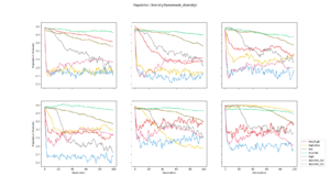 This diversity metric resulted in a scaled version of Pairwise Hamming, but took only 36 seconds to generate. See description below | 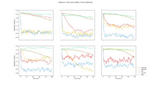 Calculated by averaging the euclidean distance between every genotype in a generation, and a "centroid genotype". The plot was generated in 40 seconds |
- Pair-wise Hamming distance
Pair-wise hamming distance is calculated by counting the number of similar genes between every pair of genomes in a population.
Failed to parse (Missing texvc executable;
please see math/README to configure.): \delta = \frac{1}{2\pi^{\frac{n}{2}}*|\Sigma|^{\frac{1}{2}}}*exp\bigg((-0.5)*\frac{(I(n,m) - \mu)'}{\Sigma}*(I(n,m) - \mu)\bigg)
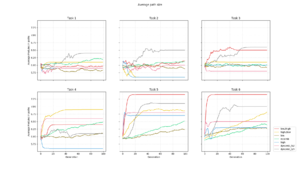
Home-made for each layer
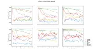
 Average population diversity for each layer in generation. Experiment: Recomb | 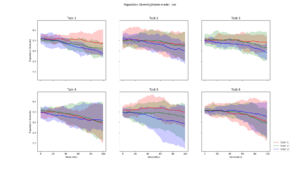 Average population diversity for each layer in generation. Experiment: Low | 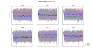 Average population diversity for each layer in generation. Experiment: High |
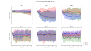 Average population diversity for each layer in generation. Experiment: Low to High | 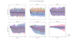 Average population diversity for each layer in generation. Experiment: High to Low |
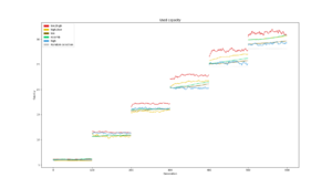
Path size
 The change in average path size for each generation. | 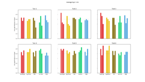 The average size of each layer in each optimal path found. |
Capacity and Reuse
 Average number of modules used during the different searches plotted consecutively. The gray dotted line is what number of modules would be used if modules were selected randomly for each task. | 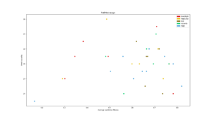 Used capacity in a PathNet plotted against that networks average classification accuracy for all tasks | 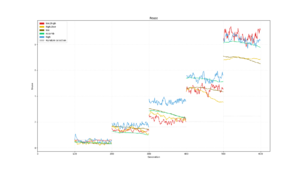 Average reuse for each generation plotted for each experiment type. The gray dotted line is what reuse would be reached by random module selection |
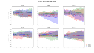
Training
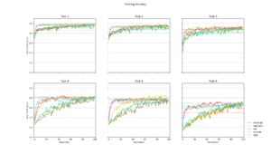 Average training accuracy for each of the five search algorithms during the search for each task. The dotted line is the validation accuracy reached after the search was completed. | 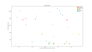 Number of training iterations in total for all modules in the PathNet plotted against the cumulative validation accuracy reached for all tasks. The size of the circle corresponds to the amount of modules used. | 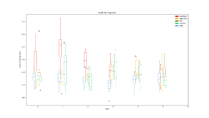 Plot of the ratio of unit training in locked and stored modules on the total number of unit training in all modules for each task |


